Random Forest and Gradient Boosted Decision Trees

Introduction

In this lecture, we will cover two popular machine learning algorithms: random forests and gradient boosting tree models. These algorithms are both ensemble methods, which means that they combine multiple weak learners to create a single strong learner. Random forests are made up of decision trees, while gradient boosting tree models are made up of decision stumps.

We will discuss the advantages and disadvantages of both algorithms, as well as how to choose the right one for your particular problem. We will also provide some guidance on how to use these algorithms in practice.

Recap: Trees and Ensembles

• Decision Trees
  • single tree-based models that split data based on rules (relational comparisons)
• Ensemble Methods
  • combine multiple models to improve performance (lower variance and bias)
  • Bagging
    • bootstrap sample the data to create multiple models, then combine their predictions
  • Boosting
    • adds simple models (called weak learners) to the ensemble by focusing on data points that were misclassified by the ensemble in previous steps

Random Forests : What are they?

Random forests are a type of ensemble method that uses decision trees as the weak learners.

Each tree in a random forest is trained on a randomly selected subset of the data, and the predictions from all of the trees are then combined to make a final prediction.

• It is also common to choose a random subset of the features to train each tree. This makes them more robust when the dimensionality is high.

Random forests are known for their accuracy and robustness.

They can be used for both classification and regression tasks.

How do random forests work?

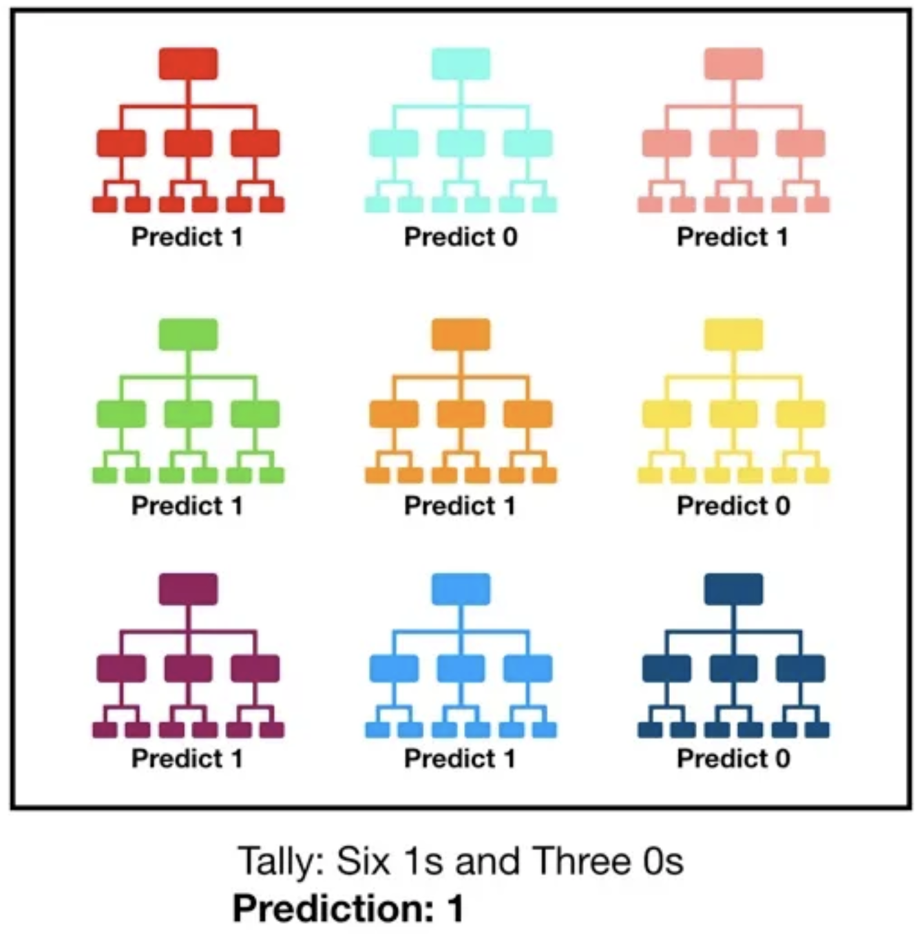
Random forests work by building a number of decision trees on a randomly selected subset of the data. The trees are then combined to make a final prediction.

The trees are built in a recursive manner. At each step, the tree is split into two branches based on a randomly selected feature. The splitting process continues until all of the data points in a branch have the same label.

The predictions from all of the trees are then combined to make a final prediction. The most common way to do this is to average the predictions from all of the trees.

Image: https://towardsdatascience.com/understanding-random-forest-58381e0602d2

Pros and Cons of Random Forests

Pros

• Can be tuned to be robust against overfitting.
• Handles missing data and outliers well.
• Suitable for high-dimensional data.
• Can handle different types of features.

Cons

• Hard to interpret the results (versus a single tree).
• Slow for large datasets.
• Can overfit if hyperparameters are not tuned correctly.
• Performance can be sensitive to the choice of hyperparameters.

Python Example

from sklearn.ensemble import RandomForestClassifier
from sklearn import datasets
from sklearn.model_selection import train_test_split

#Load dataset
iris = datasets.load_iris()
X = iris.data
y = iris.target

# Split dataset into training set and test set
X_train, X_test, y_train, y_test = train_test_split(X, y, test_size=0.3) # 70%/30% split

clf=RandomForestClassifier(n_estimators=100)

#Train the model using the training sets y_pred=clf.predict(X_test)
clf.fit(X_train,y_train)

y_pred=clf.predict(X_test)
print(y_pred)

R Example

library(randomForest)
data(iris)
set.seed(71)
trainIndex <- sample(1:nrow(iris), 100)
train <- iris[trainIndex,]
test <- iris[-trainIndex,]

rf <- randomForest(Species ~ ., data=train, ntree=500, importance=TRUE)
print(rf)

Gradient Boosted Tree Models

Gradient Boosted Decision Tree (GBDT) models are a type of ensemble method that uses either decision stumps or full decision trees as the weak learners.

• A decision stump is a one-level decision tree.¹

Each tree in a gradient boosted tree model is trained to correct the errors made by the previous trees.

Gradient boosted tree models are known for their accuracy.

They may be used for classification and regression tasks.

1. https://en.wikipedia.org/wiki/Decision_stump

How do gradient boosted tree models work?

Gradient boosted tree models work by building a number of decision stumps on the data. The stumps are then combined to make a final prediction.

The stumps are built in a sequential manner. At each step, the stump is trained to correct the errors made by the previous trees. This is done by minimizing the gradient of the loss function with respect to the predictions from the previous trees. (In other words, it tries to fit the residuals from previous trees.)

• See this blog post for an easy-to-follow description of the underlying mathematical concepts.

The predictions from all of the stumps are then combined to make a final prediction. The most common way to do this is to average the predictions from all of the stumps.

Image: Hands-On Machine Learning with R, Bradley Boehmke & Brandon Greenwell, Figure 12.1 (upscaled in Pixelmator Pro).

Pros and Cons of gradient boosted tree models

Pros

• Very accurate.
• Robust to overfitting (assuming good hyperparameter tuning).
• Suitable for high-dimensional data.
• Can handle different types of features.

Cons

• Hard to interpret the results (versus a single tree).
• Slow to train for large datasets since they train sequentially.
• Performance can be sensitive to the choice of hyperparameters, and tuning can be difficult.
• Can be sensitive to outliers.

Python Example

from sklearn.datasets import make_hastie_10_2
from sklearn.ensemble import GradientBoostingClassifier

X, y = make_hastie_10_2(random_state=0)
X_train, X_test = X[:2000], X[2000:]
y_train, y_test = y[:2000], y[2000:]

clf = GradientBoostingClassifier(n_estimators=100, learning_rate=1.0, max_depth=1, random_state=0)
clf.fit(X_train, y_train)

print(clf.predict(X_test))

R Example

library(gbm)
library(rsample)      # data splitting 
set.seed(123)
ames_split <- initial_split(AmesHousing::make_ames(), prop = .7)
ames_train <- training(ames_split)
ames_test  <- testing(ames_split)

# train GBM model
set.seed(123)
gbm.fit <- gbm(
  formula = Sale_Price ~ .,
  distribution = "gaussian",
  data = ames_train,
  n.trees = 10000,
  interaction.depth = 1,
  shrinkage = 0.001,
  cv.folds = 5,
  n.cores = NULL, # will use all cores by default
  verbose = FALSE
  )  

# print results
print(gbm.fit)

Choosing the right algorithm

So, which algorithm should you choose?

It depends on your particular problem. Simple decision trees are easier to interpret. Random forests work well on some types of problems, but more challenging problems may benefit from gradient boosted trees.

Keep in mind the scale of model complexity:
     Decision Tree \(\rightarrow\) Random Forest \(\rightarrow\) GBDT

References

Random Forest

• https://en.wikipedia.org/wiki/Random_forest
• https://towardsdatascience.com/understanding-random-forest-58381e0602d2
• Python: https://scikit-learn.org/stable/modules/generated/sklearn.ensemble.RandomForestClassifier.html
• R: https://www.r-bloggers.com/2021/04/random-forest-in-r/

Gradient Boosted Decision Trees

• https://en.wikipedia.org/wiki/Gradient_boosting
• https://towardsdatascience.com/a-visual-guide-to-gradient-boosted-trees-8d9ed578b33
• https://www.machinelearningplus.com/machine-learning/an-introduction-to-gradient-boosting-decision-trees/
• Python (Scikit-Learn):
  • Classification: https://scikit-learn.org/stable/modules/generated/sklearn.ensemble.GradientBoostingClassifier.html
  • Regression: https://scikit-learn.org/stable/modules/generated/sklearn.ensemble.GradientBoostingRegressor.html#sklearn.ensemble.GradientBoostingRegressor
• Python (XGBoost): https://xgboost.readthedocs.io/en/stable/
• Python (LightGBM): https://lightgbm.readthedocs.io/en/v3.3.2/
• R: https://www.r-bloggers.com/2017/08/gradient-boosting-in-r/

Random Forest and Gradient Boosted Decision Trees