Supervised Learning vs Unsupervised Learning
- Supervised Learning
-
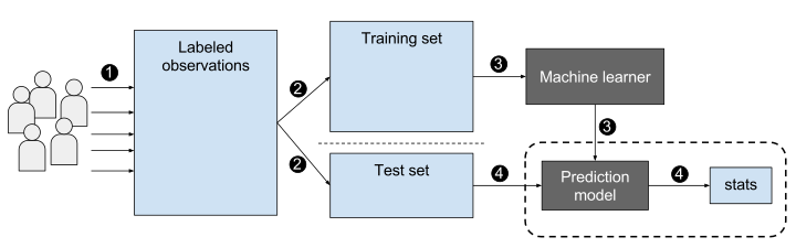
Uses labeled data to train the algorithm to make predictions or decisions. Labels come from prior knowledge (observing a result), or are provided by domain experts.
- Examples: Linear regression, decision trees, neural networks
![]()
- Unsupervised Learning
-
Uses unlabeled data to discover patterns or relationships in the data
- Examples: Clustering, Dimensionality Reduction
A key challenge in supervised learning is overfitting — when a model learns the training data too well and fails to generalize to new data.
Applications
How are supervised learning models used in different fields?
Healthcare: Predicting patient outcomes, diagnosing diseases
Finance: Credit scoring, fraud detection
Marketing: Customer segmentation, churn prediction
Automotive: Self-driving cars
Agriculture: Predicting crop yields
Security: Intrusion detection, facial recognition
Industry: Predicting supply chain issues, predicting time to failure of machine parts
Examples
Linear Regression
- Mathematical Formulation: \(y = mx + b\) or \(y = w_{0} + w_{1}x\)
- Assumptions : Linearity, independence of errors, homoscedasticity, normality, and absence of multicollinearity.
- Use Cases: Predicting housing prices, estimating sales revenue
Naive Bayes
- Probabilistic Formulation: \(P(y | x) = \frac{P(x | y)P(y)}{ P(x)}\)
- Assumptions: Conditional independence of input variables
- Use Cases: Spam filtering, sentiment analysis
Support Vector Machines
- Optimization Formulation: Maximizes the margin between the decision boundary and the closest data points
- Kernel Trick: Nonlinearly maps input variables to a higher-dimensional space to find a linear decision boundary
- Use Cases: Image classification, text classification
Examples
Decision Trees
- Structure: Tree-like structure with nodes and branches
- Interior nodes represent a decision, leaves represent a result
- Construction: Recursive partitioning of the input space based on the input variables
- Use Cases: Credit scoring, medical diagnosis
Random Forests
- Ensemble Learning: Combines multiple decision trees to improve performance and reduce overfitting
- Advantages: Robust to noise and outliers, can handle high-dimensional data
- Use Cases: Predicting customer churn, detecting credit card fraud, medical diagnosis
Examples
Neural Networks
- Architecture: Consists of layers of interconnected nodes (neurons). A neuron is a linear equation composed with a nonlinear activation \(\phi\): \(y = \phi(w_{0} + w_{1}x)\)
- Activation Functions: Nonlinear functions that introduce nonlinearity into the model, used to allow models to fit more complex data
- Use Cases: Speech recognition, image recognition
Deep Learning
- Architecture: Consists of multiple layers of neural network (i.e. more than one “hidden layer”).
- Advantages: Can learn complex patterns in the data, can handle high-dimensional data
- Use Cases: Natural language processing, computer vision
Evaluation Metrics for Classification
How do we measure and communicate the performance characteristics of classification models?
Some common metrics for classifiers are:
For all of these metrics, higher scores are considered better.
Confusion Matrix
A confusion matrix summarizes the prediction results of a classifier across all classes.
| Actual Positive |
True Positive (\(TP\)) |
False Negative (\(FN\)) |
| Actual Negative |
False Positive (\(FP\)) |
True Negative (\(TN\)) |
| \(TP\): correctly predicted positive |
\(TN\): correctly predicted negative |
| \(FP\): predicted positive, actually negative |
\(FN\): predicted negative, actually positive |
All classification metrics that follow are derived from these four counts.
Accuracy
Accuracy measures the proportion of correct predictions made by the model over the total number of predictions.
Formula: \[
\operatorname{acc} = \frac{TP + TN}{TP + FP + TN + FN}
\ \ \ \text{or}
\ \ \ acc = \frac{Correct\ Labels}{Total}
\]
Use case: Useful when classes are balanced and there is no significant cost associated with incorrect predictions. Also easiest to interpret in binary (2-class) problems.
Limitations: Can be misleading in cases where classes are imbalanced, and doesn’t take into account the cost of false positives or false negatives.
Precision and Recall
These two metrics that are often used together to evaluate the performance of a binary classifier.
Precision measures the proportion of true positives out of all predicted positives (i.e. how many of the predicted positives are actually positive)
Recall measures the proportion of true positives out of all actual positives (i.e. how many of the actual positives were correctly identified by the model)
Formulas: \[Precision = \frac{TP}{TP + FP}\] \[Recall= \frac{TP}{TP+FN}\]
Use case: Useful when classes are imbalanced or when false positives and false negatives have different costs.
Limitations: Optimizing for one metric (e.g. precision) can lead to suboptimal performance on the other metric (e.g. recall).
F1 score
The F1 score is a single metric that balances precision and recall.
Formula: \[\frac{2\times Precision \times Recall}{Precision + Recall}\ \ \ \text{or}\ \ \ \frac{\mathrm{TP}}{\mathrm{TP}+\frac{1}{2}(\mathrm{FP}+\mathrm{FN})}\]
Use case: Useful when optimizing for both precision and recall is important.
Limitations: Assumes that precision and recall are equally important, which may not always be the case.
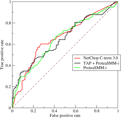
Receiver Operating Characteristic (ROC) curve
The Receiver Operating Characteristic (ROC) curve is a graphical plot that illustrates the trade-off between true positive rate (\(TPR\)) and false positive rate (\(FPR\)) for different classification thresholds.
Interpretation: The closer the curve is to the upper left corner of the plot, the better the model’s performance.
Use case: Useful when optimizing for a specific \(TPR\) or \(FPR\), or when comparing the performance of different classifiers.
Limitations: May be less informative when classes are imbalanced or when the cost of false positives and false negatives is different.
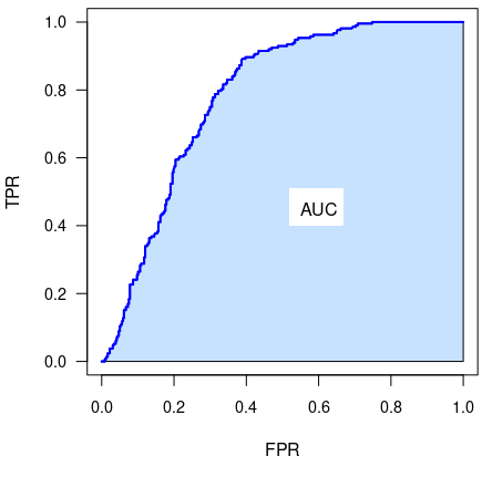
Area Under the ROC Curve (AUC or AUROC)
The area contained under the ROC curve (in the range \([0,1]\)) is often used as a performance metric. This single number describes the overall performance of a classifier model and has a range \([0,1]\).
Models whose ROC curve is “better” (in the sense of reaching closer to the upper-left) will also have a higher AUROC value.
![]()
The same limitations apply as for the ROC curve itself: The AUROC score may be less informative when classes are imbalanced or when the cost of false positives and false negatives is different.
Evaluation Metrics for Regression
Evaluating a regression model involved determining how well the expected numeric outputs match the model’s predictions. This is often (but not always) measured with a difference metric, where smaller is better.
Common regression metrics include:
Mean squared error (MSE) Lower is better.
Root mean squared error (RMSE) Lower is better.
Mean absolute error (MAE) Lower is better.
R-squared (\(R^2\) or R2) Higher is better.
Mean Squared Error (MSE)
Mean Squared Error (MSE) is the average of the squared differences between the predicted and actual values. Lower is better.
- Formula: \[MSE = \frac{1}{n} \sum_i (y_i - \hat{y}_i)^2\] Where \(y_i\) is the true value and \(\hat{y}_i\) is the predicted value.
- Use case: Useful for measuring the overall accuracy of a regression model.
- Limitations: The scale of the metric is not intuitive and may be affected by outliers.
Root Mean Squared Error (RMSE)
Root Mean Squared Error (RMSE) is the square root of the MSE between the predicted and actual values. Lower is better.
- Formula: \[RMSE = \sqrt{MSE} \ \ \ \text{or} \ \ \ RMSE = \sqrt{\frac{1}{n} \sum_i (y_i - \hat{y}_i)^2}\] Where \(y_i\) is the true value and \(\hat{y}_i\) is the predicted value.
- Use case: Useful for interpreting the magnitude of the error in the same units as the original data.
- Limitations: May be affected by outliers.
Mean absolute error (MAE)
Mean Absolute Error (MAE) is the average of the absolute differences between the predicted and actual values. Lower is better.
Formula: \[MAE = \frac{1}{n} \sum_i{|y_i - \hat{y}_i|}\]
Use case: Useful for interpreting the magnitude of the error in the same units as the original data. More robust against outliers than MSE or RMSE. More interpretable than RMSE because it is simply the average of magnitudes of the errors.
- Limitations: Does not penalize large errors as much as MSE or RMSE due to the fact that errors are not squared in MAE.
R-squared (\(R^2\) or R2)
R-squared (\(R^2\) or R2) is a metric that measures the proportion of the variance in the dependent variable that is explained by the independent variables in the model. Higher is better.
Formula: \[R^2 = 1 - \frac{SS_{residuals}}{SS_{total}} = 1 - \frac{\sum_i\left({y}_i-\hat{y}_i \right)^2}{\sum_i\left(y_i-\bar{y}\right)^2}\]
Use case: Useful for evaluating the goodness of fit of a regression model. (i.e. how well the data fit the model)
Limitations: Can be misleading with noisy data or complex models. R-squared doesn’t tell you whether your chosen model is good or bad, nor whether the data and predictions are biased. R-squared will tend to increase as the number of independent variables increases. (This isn’t a good thing.)
Adjusted R-squared can help address this: \(1-\left(1-R^2\right) \frac{n-1}{n-p-1}\) Where \(n\) is the sample size and \(p\) is the number of independent variables.
Conclusion
Supervised learning is a type of machine learning where the algorithm learns from labeled data to make predictions or decisions.
Linear regression, Naive Bayes, decision trees, random forests, support vector machines, neural networks, and deep learning are all common supervised learning models/techniques.
Each model has its own strengths and weaknesses, and should be selected based on the specific task and data.
Supervised learning has many practical applications in various industries, including healthcare, finance, and marketing.
There are several metrics for measuring the performance of regression models, each with advantages and limitations which must considered when choosing the right metric for the application.