Principal component analysis (PCA) is a statistical procedure that uses an orthogonal transformation to convert a set of observations of possibly correlated variables (entities each of which takes on various numerical values) into a set of values of linearly uncorrelated variables called principal components.1
What PCA is used for
The transformation computed by PCA serves two main purposes: Orthogonal Projection and Weighting Feature Importances.
Orthogonal Projection
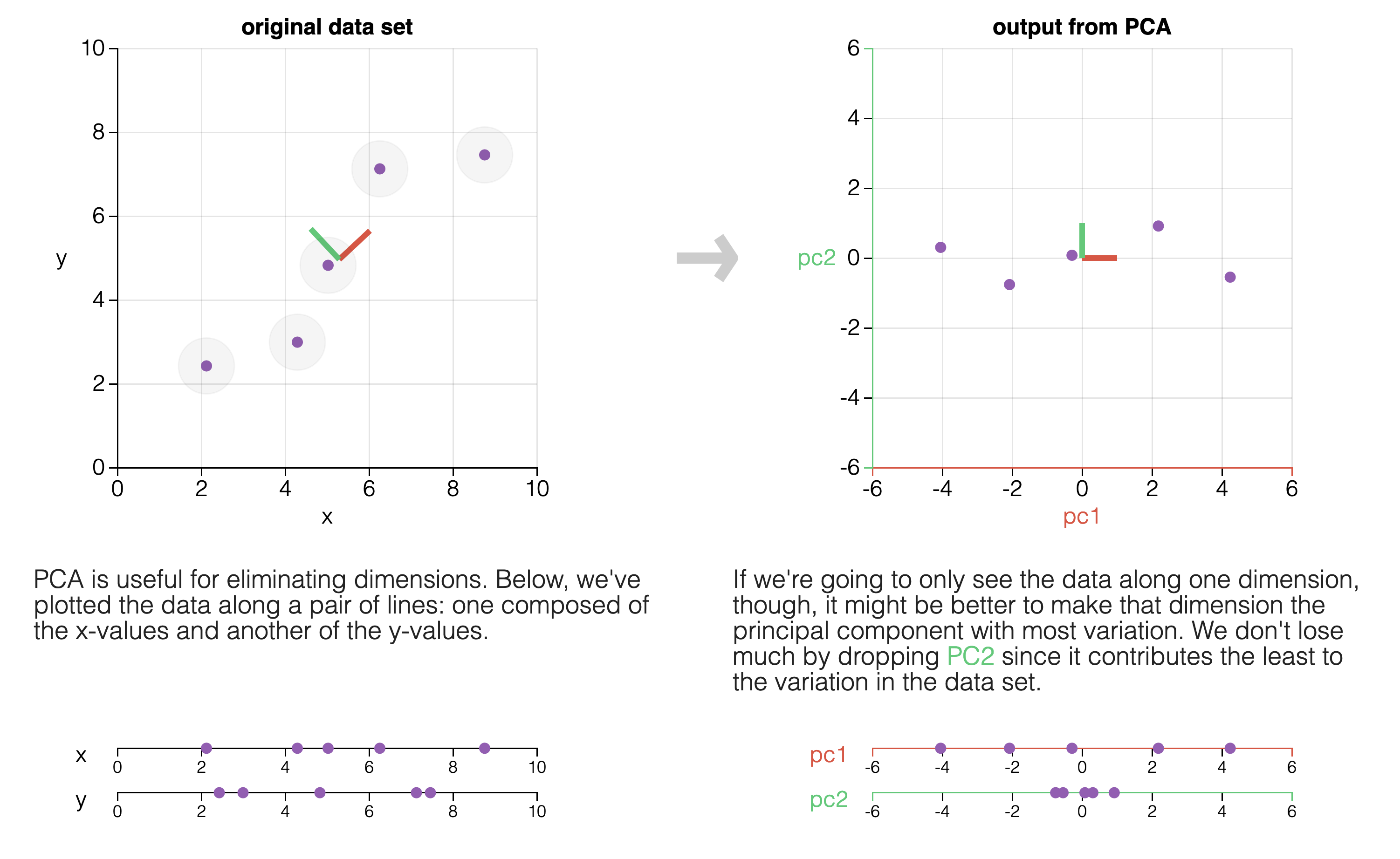
Useful for eliminating linear correlations between random variables in a dataset.
Weighting Feature Importances
Useful for explaining what is important in a dataset (from the point-of-view of explaining the variance).
Useful for dimensionality reduction, since you can keep only the most important components while maintaining most of the predictive ability of the full dataset.
What PCA Does
Given a \(n\times p\) data matrix \(\mathbf{X}\), the transformation is defined by a set of p-dimensional vectors of weights or coefficients \(\mathbf {w}_{(k)}=(w_{1},\dots ,w_{p})_{(k)}\) that map each row vector \(\mathbf{x}_{(i)}\) of \(\mathbf{X}\) to a new vector of principal component scores \(\mathbf {t}_{(i)}=(t_{1},\dots ,t_{l})_{(i)}\), given by
\[
t _ { k ( i ) } = \mathbf { x } _ { ( i ) } \cdot \mathbf { w } _ { ( k ) } \quad \text { for } \quad i = 1 , \ldots , n \quad k = 1 , \ldots , l
\]
in such a way that the individual variables \(t_1 , ... , t_l\) of \(\mathbf{t}\) considered over the data set successively inherit the maximum possible variance from \(\mathbf{x}\), with each coefficient vector \(\mathbf{w}\) constrained to be a unit vector.
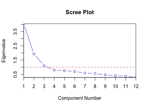
A Scree Plot is a line plot of the eigenvalues of factors or principal components in an analysis. The scree plot is used to determine the number of factors to retain in an exploratory factor analysis (FA) or principal components to keep in a principal component analysis (PCA).
Image: by Staticshakedown - Own work, CC BY-SA 4.0, https://commons.wikimedia.org/w/index.php?curid=75715167
PCA is often performed by computing the eigendecomposition1 of the matrix \(\textbf{X}\), or using the singular value decomposition (SVD)2 of \(\textbf{X}\).
Dimensionality reduction is the process of reducing the number of random variables under consideration, by obtaining a set of principal variables. It can be divided into feature selection and feature extraction.1
Since PCA computes an orthogonal basis for the dataset and also orders that basis by the amount of covariance explained by each component, it is possible to perform dimensionality reduction by selecting the first \(N\) principal components that explain enough of the variance to satisfy your needs (perhaps 95%). Then, only use those PCs for the downstream analysis.
from sklearn.decomposition import PCA# ...# ... Let X = the random variables you want to compute the PCA for.# This will keep only the first two principle componentspca = PCA(n_components=2)pca.fit(X)# Print some infoprint(f"Explained variance: {pca.explained_variance_ratio_}")print(f"Singular values: {pca.singular_values_}")
#| echo: true# Load the Iris datasetdata(iris)log.ir <-log(iris[, 1:4]) # log transformir.species <- iris[, 5] # get the species column# Apply PCA# `scale.` will apply standardization before the PCA computation.# Setting `scale. = TRUE` is often recommended, but default is FALSE.ir.pca <-prcomp(log.ir,center =TRUE,scale. =TRUE)# Prints an information table for the results:print(ir.pca)