Statistical Distributions
Part 2
Communicating Effect Size
Statistical significance tells you how unlikely it is that something is due to chance, but not whether it is important.
In particular, significance does not communicate anything about effect size.
We saw that even very small effects can be “significant” (w.r.t. a fixed choice of \(\alpha\)) given large enough sample sizes.
There are several methods to measure effect size, where we will generally consider small effects to be difficult to observed unaided, medium effects to be visible to a careful human observer, and large effects to be obvious.
Cohen’s \(d\)
Cohen’s \(d\) bases importance on the magnitude of the change in means, and also the natural variation in the distributions: \[ d = \frac{\left( \left| \mu - \mu^\prime \right| \right)}{\sigma} \] A reasonable threshold for a small effect size is \(> 0.2\), medium effect \(> 0.5\), and large effect size \(> 0.8\).
The \(\sigma\) in the denominator is often the pooled standard deviation.
Pearson’s correlation coefficient \(r\)
Pearson’s correlation coefficient \(r\) measures the degree of linear relationship between two variables, on a scale from -1 to 1.
The thresholds for effect sizes are comparable to the mean shift: small effects start at \(\pm 0.2\), medium effects at \(\pm 0.5\), and large effects at \(\pm 0.8\).
The coefficient of variation \(r^2\)
The coefficient of variation \(r^2\): is the square of the correlation coefficient.
It reflects the proportion of the variance in one variable that is explained by the other.
The thresholds follow from squaring those above. Small effects explain at least 4% of the variance, medium effects \(\geq 25\%\) and large effect sizes at least 64%.
Percentage of overlap
The area under any single probability distribution is, by definition, 1.
The area of intersection between two given distributions (Percentage of overlap) is a good measure of their similarity.
Identical distributions overlap 100%, while disjoint intervals overlap 0%.
Reasonable thresholds are: for small effects 53% overlap, medium effects 67% overlap, and large effect sizes 85% overlap.
Comparing Population Means: The T-test
We have seen that large mean shifts between two populations suggest large effect sizes. But how many measurements do we need before we can safely believe that the phenomenon is real?
The \(t\)-test evaluates whether the population means of two samples are different.
The T-test
Two means differ significantly if:
- The mean difference is relatively large.
- The standard deviations are small enough.
- The number of examples are large enough.
The t-test computes a test statistic on the two sets of observations.
t-test Test Statistic
Welch’s t-test
Assuming Normally distributed variables.
\[ t=\frac{\overline{x}_{1}-\overline{x}_{2}}{\sqrt{\frac{\sigma_{1}^{2}}{n_{1}}+\frac{\sigma_{2}^{2}}{n_{2}}}} \] where \(\overline{x}_{i}\), \(\sigma_i\), and \(n_i\) are the mean, standard deviation, and population size of sample \(i\), respectively.
Student’s t-test
You may have heard of Student’s t-test (it is more often taught in Stats classes). It assumes normal distributions with equal variances; the Welch’s t-test allows for unequal variances, so it is a bit more robust.
“Student” was actually the pen name of William Sealy Gosset, who was a chemist at the Guinness brewery in 1908 when he was publishing; Guinness did not allow their scientists to publish under their real names.
Interpreting the t-statistic
Interpreting the meaning of a particular value of the t-statistic comes from looking up a number in an appropriate table. For a desired significance level \(\alpha\) and number of degrees of freedom (essentially the sample sizes), the table entry specifies the value \(v\) that the t-statistic \(t\) must exceed. If \(t > v\), then the observation is significant to the \(\alpha\) level.
t-tests in Code
The R language provides the t.test() function that will perform a Welch’s t-test.
In Python, you can use scipy.stats.ttest_ind(), which can do either Student’s or Welch’s test.
See the example at:
https://pythonfordatascienceorg.wordpress.com/welch-t-test-python-pandas/
Testing Assumptions
Many statistical tests (like the t-test) assume the variables are Normally distributed. You should check by both observing the distribution (plot it, do a boxplot, plot residuals from mean, plot a Q-Q plot), and by testing with a test like Shapiro’s test.
In R: shapiro.test( ... )
In Python: scipy.stats.shapiro( ... )
Kolmogorov-Smirnov Test
What if your data isn’t Normal?
The t-test compares two samples drawn from presumably normal distributions according to the distance between their respective means.
Instead, the Kolmogorov-Smirnov (KS) test compares the cumulative distribution functions (cdfs) of the two sample distributions and assesses how similar they are.
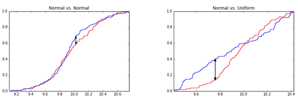
The Kolmogorov-Smirnov test quantifies the difference between two probability distributions by the maximum \(y\)-distance gap between the two cumulative distribution functions.
Kolmogorov-Smirnov Test in Code
R: ks.test( ... )
Python: scipy.stats.kstest( ... )
How can this go wrong?
- Type I Error
- A Type I error in hypothesis testing means that you have mistakenly rejected a null-hypothesis. In other words, the null hypothesis was true, but your hypothesis test showed high enough significance (low enough “p-value”) that you chose to reject the null hypothesis. This is also called a false positive result.
- Type II Error
- A Type II error in hypotheses testing means that you have mistakenly failed to reject the null-hypothesis. In other words, the alternative hypothesis was true, but your hypotheses test failed to achieve significance, so you did not reject the null hypothesis. This is also called a false negative result.
Multiple Testing: Beware
If you perform the same test multiple times, your chance of committing a Type I error increases.
Why? Remember that in hypothesis testing, the \(\alpha\) threshold represents the likelihood of observing your evidence, given that the null hypothesis holds. In other words, \(\alpha\) is the chance that your test could result in a Type I error.
If we pick \(\alpha = 0.05\) as our significance threshold, we have a \(\frac{1}{20}\) chance of Type I error for a single test.
Multiple Testing: Beware
If we pick \(\alpha = 0.05\) as our significance threshold, we have a \(\frac{1}{20}\) chance of Type I error for a single test.
If the null hypothesis is true, the probability of not obtaining a significant result (i.e. no Type I error) is:
\[ \text{prob. of not having Type I error} = 1 - 0.05 = 0.95 \]
So, if the null hypothesis is true, the probability of obtaining a significant result (i.e. Type I error) is:
\[ \text{prob. of Type I error} = 1 - 0.95 = 0.05 \]
Which is exactly the definition of \(\alpha = 0.05\) to begin with.
Multiple Testing: Beware
But, let’s say we perform the test 5 times.
Each test has a 0.95 probability of not producing a Type 1 error, so 5 tests have a \(0.95^5\) chance of not producing a Type 1 error.
\[ \text{prob. of not having Type I error} = 0.95^5 \approx 0.77 \]
Our chances of Type I error are now:
\[ \text{prob. of Type I error} = 1 - 0.95^5 \approx 0.23 \]
What if we do 10 tests?
\[ \text{prob. of Type I error} = 1 - 0.95^{10} \approx 0.40 \]
The Bonferroni Correction
The Bonferroni correction provides an important balance in weighing how much we trust an apparently significant statistical result. It speaks to the fact that how you found the correlation can be as important as the strength of the correlation itself.
When we repeat a test many times, the odds of observing a rare event are increased. This doesn’t mean it should be considered significant.
The Bonferroni correction states that when testing \(n\) different hypotheses simultaneously, the resulting \(p\)-value must rise to a level of \(\frac{\alpha}{n}\) in order to be considered as significant at the \(\alpha\) level.
Reference Links
Hypothesis Testing Example
https://towardsdatascience.com/hypothesis-testing-in-real-life-47f42420b1f7
Multiple Testing
http://grants.hhp.coe.uh.edu/doconnor/PEP6305/Multiple%20t%20tests.htm
https://www.stat.berkeley.edu/~hhuang/STAT141/Lecture-FDR.pdf
Bonferroni Correction
https://toptipbio.com/bonferroni-correction-method/
Appendix
The following is the python code and annotations used to produce the uniform sampling within a circle example figures. It has been split into “slides” to match the format of the document, and the data marker sizes and figure sizes have been scaled down to fit on the slides.
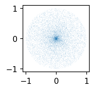
What if we generate an angle \(\Theta\) and distance \(d\) from the center at random?
Monte Carlo sampling method
- Draw a random (uniform) (x,y) point within -r and r in each direction.
- See if the point falls within r units of the circle’s center; if so, keep it; if not, reject it.
Let’s generate a lot of points and plot them:
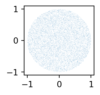
That is much better!

Statistical Distributions

CS 4/5623 Fundamentals of Data Science