Mathematical Preliminaries

Part 1

Material herein is from from The Data Science Design Manual, Chapter 2, with introductory material from Introduction to Machine Learning (Adaptive Computation and Machine Learning series) by Ethem Alpaydin.

A data scientist is someone who knows more statistics than a computer scientist and more computer science than a statistician. — Josh Blumenstock

– The Data Science Design Manual, Chapter 2.

Types of variables

categorical: A variable that is allowed to take on only a finite (usually small) set of values. Categorical variables are usually non-numeric, but are sometimes encoded as numbers. R refers to values of this type as factors.
discrete: (or integral) A numeric variable that can only take on whole-number values.
continuous: A variable that can take on any value between two numbers.

A free reference for types of variables:
https://www.mayo.edu/research/documents/data-types/doc-20408956

Other ways of describing variable types

nominal: Categorical values; can be compared for equality, but no ordering is implied.
Examples: ID numbers, eye color, zip codes
ordinal: Categorical values (but may be numbers); can be compared for equality and ranked with \(>,\geq,<,\leq\)
Examples: rankings (e.g., taste of potato chips on a scale from 1-10), grades, height {tall, medium, short}
interval: Numeric or number-like, discrete or continuous; meaningful operations include addition, subtraction (can express ranges).
Examples: calendar dates, temperatures in Celsius or Fahrenheit.
ratio: Numeric, usually continuous; meaningful operations include ratios (multiplication/division makes sense); has a defined “origin”.
Examples: temperature in Kelvin, length, time, counts

Representing values we don’t know ¹

Missing: Missing data are data that are missing and you don’t know the mechanism. You should use a single common code for all missing values (for example, “NA”), rather than leaving any entries blank.
Censored: Censored data are data where you know something about the mechanism responsible for the data being absent. Common examples are a measurement being below a detection limit or a patient leaving a study before their follow-up appointment. They should also be coded as “NA” when you don’t have the data. But you should also add a new column to your data called e.g. “VariableNameCensored” which should have values of TRUE if censored and FALSE if not.

It is important to know whether a value is missing or censored, as statistical approaches for handling each are different.

Goals of a Data Analysis

Understanding existing data
- Visualizations
- Tables
- Reports
Making Decisions (predicting future outcomes)
- Classification
- Regression

The data analysis question type flow chart¹

How much math?

We assume that as a student in this class, you have:

Some degree of exposure to probability and statistics, linear algebra, and continuous mathematics.
- (You may have forgotten some or even most of it.)
You are prepared to pull out old textbooks or do some self-guided learning online to fill in missing details.

Classification

classification: Input variables are used to determine a categorical output value.
discriminant: a function that separates the examples of different classes.
prediction: Given a new set of input variables, a prediction function gives the expected output based on the model.

Classification (red vs blue).

Image: Mekeor, CC BY-SA 3.0 https://creativecommons.org/licenses/by-sa/3.0, via Wikimedia Commons

Regression

When we want to use the input variables to predict a numeric value (especially a continuous value), we have a regression problem.

A simple example is a linear model such as:

\[ y = w_0 + w_1 x \]

Where the coefficients \(w_0\) and \(w_1\) will also be referred to as weights.

Regression

Image: Cdang, CC0, via Wikimedia Commons

knowledge extraction

Once we have learned a rule from data, the rule is a simple model that explains the data — looking at this model we have an explanation about the process underlying the data.

Once we have a rule separating low-risk and high-risk loan customers, we have knowledge of the properties of low-risk customers.

compression

In a way, learning a model also performs compression in that the model is simpler than the original data, requiring less memory to store and (maybe) less computation to process.

outlier detection

finding instances that do not obey the general rule and are exceptions. Typical instances share characteristics that can be simply stated and instances that do not have those characteristics are atypical. (may also be viewed as novelty detection)

Probability

Probability theory gives us a formal framework for reasoning about the likelihood of events. Like all formal disciplines, it comes with its own technical jargon:

An experiment is a procedure which yields one of a set of possible outcomes. (Tossing a 6-sided die, for example.)

A sample space S is the set of possible outcomes of an experiment. (Tossing a six-sided die has six possible outcomes.)

An event E is a specified subset of the outcomes of an experiment. (The event that the die results in an even value = \({2, 4, 6}\))

The probability of an outcome s, denoted by \(p(s)\) is a number with the properties:
1. For each outcome \(s\) in sample space \(S\), \(0 \le p(s) \le 1\).
2. The sum of probabilities of all outcomes adds to one: \(\sum_{s\in S} p(s) = 1\).

Probability (continued)

The probability of an event E is the sum of the probabilities of the outcomes of the experiment:
\(P(E) = \sum_{s\in E} P(s)\)

You can also look at the relationship between \(P(E)\) and its complement (\(\bar{E}\)) — the case where \(E\) does not occur:
\(P(E) = 1 - P(\bar{E})\)

A random variable V is a numerical function on the outcomes of a probability space. Example: “sum the values of two dice” (\(V((a,b)) = a+b\)) produces an integer result in the range \([2,12]\). The probability \(P(V(s) = 7) = \frac{1}{6}\), while \(P(V(s) = 12) = \frac{1}{36}\).

The expected value \(E(V)\) of a random variable \(V\) defined on a sample space \(S\), is defined:
\(E(V) = \sum_{s\in S} P(s) \cdot V(s)\)

Probability vs. Statistics

Probability deals with predicting the likelihood of future events, while statistics involves the analysis of the frequency of past events.
Probability is primarily a theoretical branch of mathematics, which studies the consequences of mathematical definition. Statistics is primarily an applied branch of mathematics, which tries to make sense of observations in the real world.

Many a gambler has gone to a cold and lonely grave for failing to make the proper distinction between probability and statistics.
— Steven S. Skiena

Probability theory enables us to find the consequences of a given ideal world, while statistical theory enables us to measure the extent to which our world is ideal.

de Méré’s Dice

1654, France: Chevalier de Méré is interested in a dice game.

Player rolls 4 6-sided dice.
- House wins if any of them are a 6.
- Player wins otherwise.

de Méré’s Dice

Player rolls 4 6-sided dice.
- House wins if any of them are a 6.
- Player wins otherwise.

Each roll: \(V(s) = 6 = \frac{1}{6}\).

With 4 rolls, there are \(6^4\) possible outcomes. You win with \(5^4\) of them.

You win with \(p=(\frac{5}{6})^4\), so the house’s chance of winning is:
\(p=1-(\frac{5}{6})^4 \approx 0.5177\)

(A fair game would have \(p=0.5\).)

(NOTE: Thank Pascal for figuring this out.)

See https://mathworld.wolfram.com/deMeresProblem.html

Compound Events and Independence

The problem: Computing complex events from a set of simpler events \(A\) and \(B\) on the same set of outcomes.

Set theory is important here. Given \(A\) and \(B\),

\(\bar A\) : complement of \(A\). \(\bar A = S - A\)

\(A\cup B\) : union of \(A\) and \(B\).

\(A\cap B\) : intersection of \(A\) and \(B\). \(A\cap B = A - (S - B)\)

\(A-B\) : set difference of \(A\) and \(B\).

Two events \(A\) and \(B\) are independent if and only if:

\[P(A\cap B) = P(A) \times P(B)\]

Probability theorists love independent events, because it simplifies their calculations. But data scientists generally don’t. […]
Correlations are the driving force behind predictive models.
— Steven S. Skiena (emphasis mine)

Conditional Probability

When two events are correlated, there is a dependency between them which makes calculations more difficult. The conditional probability of \(A\) given \(B\), \(P(A|B)\) is defined as:

\[ P(A|B) = \frac{P(A\cap B)}{P(B)} \]

Example: Roll 2 6-sided dice. (36 outcomes)
\(A\): at least one of two dice is an even number. (27 ways)
\(B\): the sum of the two dice is either 7 or 11. (8 ways)

\(P(A|B) = 1\) since any roll resulting in an odd value required one odd and one even number. So \(A\cap B = B\).
For \(P(B|A)\), note that \(P(A\cap B) = \frac{8}{36}\) and \(P(A) = \frac{27}{36}\), so \(P(B|A) = \frac{8}{27}\).

Bayes’ theorem

The primary tool we will use to compute conditional probabilities is Bayes’ Theorem:

\[ P(B|A) = \frac{P(A|B)P(B)}{P(A)} \]

Using the previous example, \(P(B|A) = (1\cdot \frac{8}{36}) / (\frac{27}{36}) = \frac{8}{27}\).

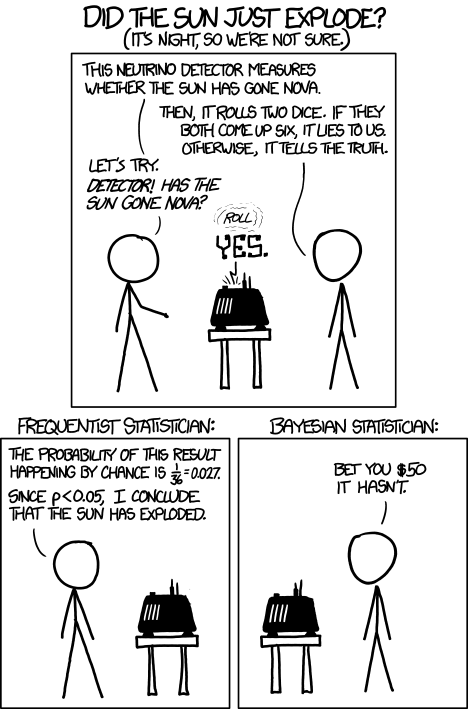
Frequentists vs. Bayesians

Image: https://xkcd.com/1132

Probability Distributions

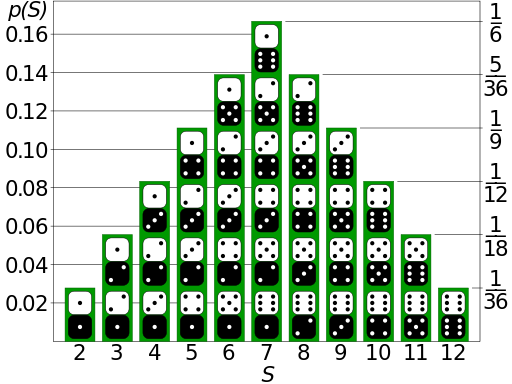
Random variables are numerical functions where the values are associated with probabilities of occurrence.

They can be represented by their probability density function, or pdf. In graph form, x-axis represents the range of values the random variable can take on, and y-axis represents the probability of that given value.

Sum of 2d6

Probability Distributions (continued)

pdf graphs are related to histograms of data frequency. To convert a histogram to a pdf, divide by the total frequency.

Histograms are statistical: They represent the actual observations of outcomes. Pdf’s are probabilistic: They represent the underlying chance that the next observation will have the value X.

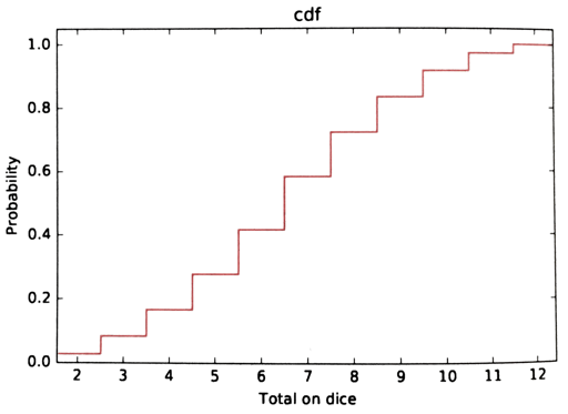
The cumulative density function, or cdf is the running sum of the probabilities in the pdf. As a function of \(k\), it represents the probability that \(X < k\).

Sum of 2d6 (cdf)

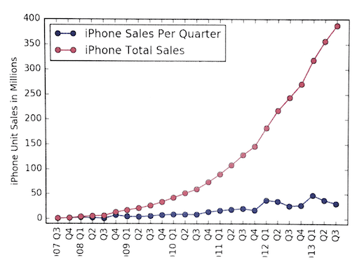
iPhone Sales Per Quarter

Which line would you show off?

They are the same!

Mathematical Preliminaries